From BigQuery to Snowflake: What a Real-World Analytics Migration Actually Looks Like

There’s a version of this story that gets told a lot. A team decides to migrate their analytics workload from one cloud data warehouse to another. They write a few scripts, move some data, update some connection strings, and call it done.

That version is fiction.

Here’s what it actually looked like when I recently led a migration of an analytics platform from BigQuery to Snowflake for a large-scale e-commerce organisation — moving a production workload that feeds live PowerBI dashboards used by multiple teams across the business.

Why We Migrated

The organisation had its source-of-truth data in BigQuery, processed through a well-established dbt pipeline. But the downstream analytics consumers — the teams building dashboards, running ad-hoc queries, training ML models — were being onboarded to a Snowflake ecosystem that was becoming the standard data platform across the organisation.

The decision wasn’t about one platform being better than the other. It was about meeting the consumers where they already were, and aligning with the organisation’s broader data platform strategy.

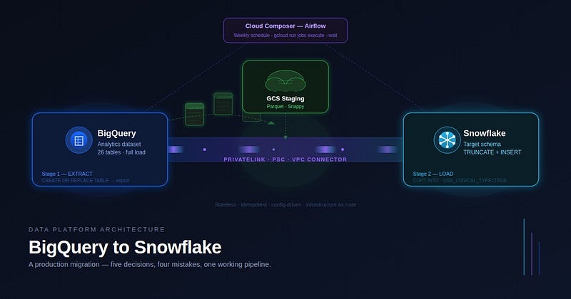
The requirement was clear: take approximately 30 tables from a BigQuery mart dataset and make them available in a Snowflake schema, refreshed weekly, reliable, and production-grade.

The Architecture We Built

After evaluating the options, we landed on a three-stage extract-stage-load pattern using GCS as an intermediate layer.

┌─────────────────────────────────────────────────────────┐
│                                                         │
│  Cloud Composer (Airflow)                               │
│  — schedules weekly on Monday 06:00 UTC                 │
│         │                                               │
│         ▼                                               │
│  Cloud Run Job (containerised Python)                   │
│         │                                               │
│    ┌────┴────────────────────────────────┐              │
│    │                                     │              │
│    ▼                                     ▼              │
│  BigQuery                            Snowflake          │
│  mart dataset          GCS           target schema      │
│  (source)     ───►  (Parquet)  ───►  (TRUNCATE +        │
│                     staging         INSERT)             │
│                                                         │
└─────────────────────────────────────────────────────────┘

The sequence diagram below shows exactly how these components interact across a single pipeline run:

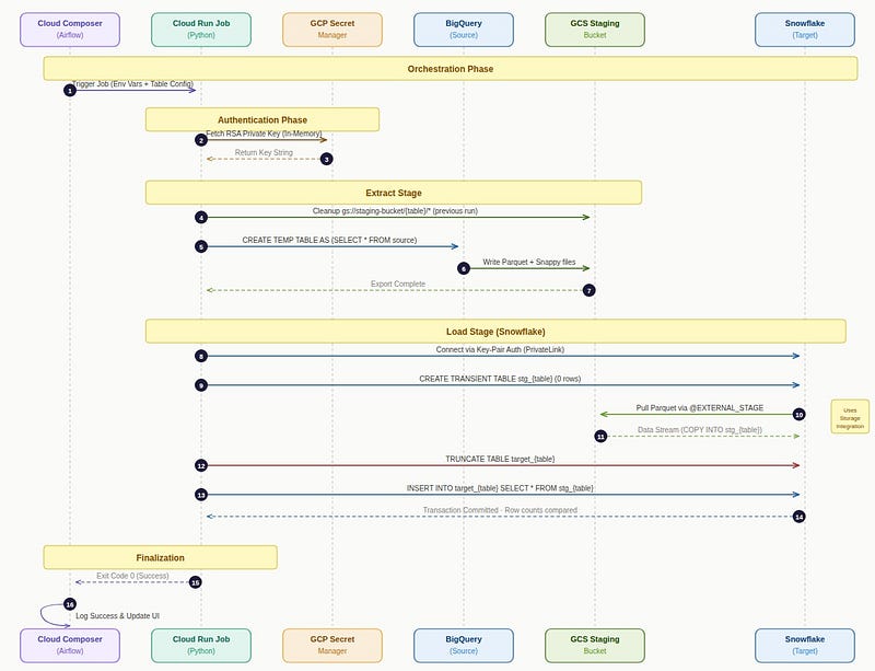
Sequence diagram for pipeline Every component in this architecture was chosen deliberately. Let me walk through the key decisions.

Decision 1: Parquet over CSV

The obvious choice for intermediate staging is CSV. It’s simple, readable, and every tool supports it.

We didn’t use it.

The reason is type fidelity. BigQuery exports timestamps as strings in CSV format, which means you need to re-cast them on the Snowflake side. Integers, floats, booleans — all become text. Each one needs careful mapping back to the correct type. Every mapping is a potential silent bug.

Parquet preserves native types end-to-end. A TIMESTAMP in BigQuery lands as TIMESTAMP_NTZ in Snowflake. A BOOL is a BOOL. An INT64 is a NUMBER. No casting, no format strings, no character encoding edge cases.

There’s also a practical lesson here that took us a while to learn: Snowflake’s COPY INTO command for Parquet needs USE_LOGICAL_TYPE = TRUE or it will misinterpret timestamp columns as raw microseconds since epoch, resulting in dates in the year 56,000. This isn't in the headline documentation. We found it the hard way, in production, looking at dashboards full of nonsense dates.

The lesson: Choose a staging format that preserves your type contract. The marginal complexity of Parquet over CSV pays for itself the first time you avoid a silent type corruption bug.

Decision 2: Cloud Run Jobs over a managed orchestration cluster

We had access to a shared GKE cluster running similar workloads. The easy path was to deploy our container there.

We didn’t do that either.

The shared cluster belonged to another team. Using it would mean a runtime dependency on infrastructure we didn’t own, didn’t control, and couldn’t modify. It would also mean that any changes to that cluster’s configuration, networking, or service accounts would require coordination across teams.

Cloud Run Jobs gave us complete ownership of our runtime. Serverless, no cluster to manage, no shared state, billed only for actual execution time. The container runs, the data moves, the job exits. Clean.

The networking decision that followed from this was more interesting: Cloud Run Jobs must be in the same region as their VPC connector. Snowflake’s PrivateLink endpoint in our setup existed in europe-west4. That meant the VPC connector had to be in europe-west4. Which meant the Cloud Run Job had to be in europe-west4. Which meant we had to create a new subnet and connector in the production project, because the existing connectors were all in europe-west1.

The lesson we learned: Serverless runtimes are not free of networking constraints. Region alignment between Cloud Run, VPC connectors, and private endpoints is a hard requirement, not a configuration detail.

Decision 3: PrivateLink over public internet

Early in testing, the Cloud Run job connected to Snowflake over the public internet. Snowflake blocked it immediately:

Incoming request with IP X.X.X.X is not allowed to access Snowflake. The organisation’s Snowflake account had a network policy restricting inbound connections. We had two options: whitelist the Cloud NAT IP, or use PrivateLink via GCP Private Service Connect.

We chose PrivateLink. The reason isn’t just security — it’s operational stability. Cloud NAT IPs can change. A whitelisted IP that gets rotated silently breaks your pipeline. PrivateLink routes traffic through a private network endpoint with a stable DNS name that resolves inside the VPC.

The setup involved creating a PSC forwarding rule pointing to Snowflake’s service attachment, a private DNS zone that resolves the Snowflake PrivateLink hostname to the PSC endpoint’s private IP, and a VPC connector in the right region to route Cloud Run traffic through the private network.

In the development environment, all of this had already been set up by a colleague’s team for a different workload. We discovered it by querying the existing infrastructure rather than creating something new. In production, none of it existed. We created it from scratch — subnet, VPC connector, PSC forwarding rule, DNS zone, A record — six sequential steps, each depending on the output of the previous.

The lesson we learned: Before building networking infrastructure, audit what already exists. In a shared GCP organisation, the resources you need are often already there for a different use case.

Decision 4: TRUNCATE + INSERT over MERGE

The natural instinct for loading data into a target table is MERGE. Find matching rows, update them. Insert new ones. Elegant, efficient.

Our target tables had no primary keys. Not a single one across 26 tables. MERGE without a join condition is not MERGE — it’s either a full cross join or a syntax error.

We chose TRUNCATE + INSERT. On every run, the target table is emptied completely and all rows are inserted fresh from the Parquet files. This is only viable because every run is a full load — we export the entire source table from BigQuery, not just changed rows.

The benefit of this approach is operational simplicity: every run is idempotent. If a run fails halfway through, the retry starts fresh. There’s no partial state, no duplicate detection, no upsert logic to reason about. The worst outcome of a failed run is that a table is empty until the next successful run.

The lesson: Full load with TRUNCATE + INSERT is not a lazy approach. It’s a deliberate trade-off that eliminates an entire class of data consistency bugs in exchange for slightly higher data latency.

Decision 5: Stateless pipeline with config-driven table list

The pipeline we adapted as a starting point used GCP Datastore to track watermarks — timestamps indicating when each table was last successfully loaded. This made sense for that pipeline, which did incremental loads.

We removed Datastore entirely. With full load, there is no watermark to track. The pipeline reads its configuration from a single JSON file in GCS, runs, and exits. No state persists between runs.

The table list lives in that config JSON:

{ "tables": [ { "name": "fact_table_1", "load_type": "full" }, { "name": "dim_table_1", "load_type": "full" } ]} Adding a new table to the pipeline requires no code change, no Docker rebuild, no deployment. Update the JSON, upload to GCS, and it takes effect on the next run.

The lesson: Stateless pipelines are easier to reason about, easier to retry, and easier to operate. If your use case allows it, remove the state.

How the Code is Structured

The pipeline is a single Python container, roughly 600 lines across a handful of modules:

src/
├── main.py                   ← orchestration — calls BQ, GCS, Snowflake in order
├── helper.py                 ← logging utilities
├── bigquery_services.py      ← BQ temp table cleanup
├── bucket_services.py        ← GCS path cleanup before each run
└── model/
    ├── MirroringConfig.py             ← dataclass loaded from the config JSON
    ├── MirroringObjectConfigs.py      ← per-table paths and table names
    └── PreparedSnowflakeColumns.py    ← column SQL for INSERT statements

The entry point in main.py follows a simple loop per table:

for table_name in full_load_tables:
    # 1. Clean previous run's GCS files
    cleanup_bucket(bucket, table_path)
    # 2. Export BQ table → GCS as Parquet/Snappy
    bq_rowcount, columns = bigquery_to_gcs(table_name, config)
    # 3. COPY INTO Snowflake temp table from External Stage
    #    FILE_FORMAT = (TYPE=PARQUET SNAPPY_COMPRESSION=TRUE USE_LOGICAL_TYPE=TRUE)
    #    MATCH_BY_COLUMN_NAME = CASE_INSENSITIVE
    # 4. TRUNCATE target table
    # 5. INSERT INTO target SELECT * FROM temp table
    # 6. Compare row counts BQ vs Snowflake
    # 7. DROP temp table

The Snowflake connection uses RSA key-pair authentication. The private key is fetched from Secret Manager at runtime and loaded directly into memory using Python’s cryptography library — the key bytes are passed straight to the Snowflake connector without ever touching disk:

private_key = serialization.load_pem_private_key(
    private_key_str.encode(),
    password=passphrase_str.encode(),
    backend=default_backend()
)
private_key_bytes = private_key.private_bytes(
    encoding=serialization.Encoding.DER,
    format=serialization.PrivateFormat.PKCS8,
    encryption_algorithm=serialization.NoEncryption()
)
ctx = snowflake.connector.connect(
    host=f"{account}.privatelink.snowflakecomputing.com",
    account=account,
    user=user,
    private_key=private_key_bytes,
    ...
)

One pattern worth noting: the Snowflake connection is reused across tables within a single run, but the code checks liveness before each table and reconnects if the session has closed. Long-running exports on large tables can outlive an idle Snowflake session.

The Infrastructure is Code. All of It.

Every GCP resource in this pipeline is managed by Terraform — a single core/ module with an env variable that drives everything:

deployment/terraform/core/
├── config.tf         ← project = "myproject-${var.env}", region, VPC connector path
├── backend.tf        ← GCS state bucket (passed via -backend-config at init time)
├── provider.tf       ← GCP provider
├── variables.tf      ← env variable (dev | prd)
├── bucket.tf         ← GCS staging bucket
├── iam.tf            ← service account, all IAM bindings
└── cloud_run_job.tf  ← Cloud Run Job with env vars, VPC access, image reference

Running terraform apply -var="env=dev" targets the dev project; terraform apply -var="env=prd" targets production. The Terraform state is stored in a separate GCS bucket per environment, switched at init time:

# dev
terraform init -backend-config="bucket=myproject-dev-tf-state"
terraform apply -var="env=dev"

# prd
terraform init -reconfigure -backend-config="bucket=myproject-prd-tf-state"
terraform apply -var="env=prd"

There’s one cross-environment dependency worth calling out: both the dev and production Cloud Run Jobs pull their Docker image from a single Artifact Registry repository in the dev project. We tag images by environment (pipeline-dev:latest, pipeline-prd:latest) but store them in one place. This means the production service account and Cloud Run Service Agent both need artifactregistry.reader on the dev registry — bindings managed in the dev Terraform state.

The consequence: always apply dev Terraform before production. The dev state creates the IAM bindings that allow production to pull the image. If you apply production first, the job will fail with a ContainerPermissionDenied error that looks like a Docker issue but is actually an IAM issue.

A Cloud Build pipeline (cloudbuild-rollout.yaml) automates the full sequence:

steps:
  - id: build-and-push
    # docker build + push for the right env tag
  - id: terraform-apply
    name: hashicorp/terraform:1.2.5
    args:
      - terraform init -backend-config="bucket=myproject-${_ENV}-tf-state"
      - terraform apply -var="env=${_ENV}" -auto-approve
  - id: upload-config
    # gcloud storage cp configs/pipeline-${_ENV}.json gs://...
  - id: deploy-dag
    # gcloud storage cp dags/pipeline_dag.py gs://airflow-bucket/dags/

The substitution _ENV is passed at trigger time — the same YAML file deploys both dev and production.

What We Got Wrong (and Fixed)

No honest architecture writeup omits the mistakes.

Timestamp misinterpretation. Parquet stores timestamps as microseconds since epoch. Snowflake interprets these correctly only when USE_LOGICAL_TYPE = TRUE is set in the COPY INTO file format. Without it, every timestamp column shows a date around year 56,000. We found this in the development environment before it reached production, but only after a full pipeline run had loaded garbage data into Snowflake tables.

VPC connector region mismatch. We initially deployed the Cloud Run Job in europe-west1 and tried to attach a VPC connector in europe-west4. Cloud Run enforces that the job and connector must be in the same region. This error is clear when you see it, but it required recreating the Cloud Run Job in a different region, which Terraform handles as a destroy-and-recreate operation.

Private key in a temp file. The original pipeline code wrote the Snowflake RSA private key to a temporary file on the container filesystem, then passed the file path to the Snowflake connector. We replaced this with in-memory key handling — the key bytes are loaded from Secret Manager directly into a cryptography library object and passed to the connector without touching disk. This is a security hygiene improvement that the original code had taken a shortcut on.

Schema name changes mid-project. The target Snowflake schema was renamed by the platform team partway through the project — from <SCHEMA_NAME>_WORKSPACE to <SCHEMA_NAME>_PROV. This required updating the stage reference, the config JSON, the Terraform IAM grants, and the Snowflake tables. The config-driven architecture meant the code itself didn't need to change, but every reference to the schema name in external resources did.

The**count = var.env == "dev" ? 1 : 0**pattern. The Artifact Registry IAM bindings for the production service account are managed in the dev Terraform state using a count condition. This means running terraform apply -var="env=prd" alone is never enough for a first-time production deployment — you have to apply dev first. We documented this, but it still caught us out once.

The Infrastructure is Code. All of It.

Every resource in this pipeline is managed by Terraform. The staging GCS bucket, the service account and its IAM bindings, the Cloud Run Job definition, the Secret Manager access grants — all of it is code, versioned, and reproducible.

The one complication: the production pipeline’s Docker image lives in Artifact Registry in the development GCP project (because Artifact Registry is expensive to duplicate). The production Cloud Run Job pulls from a registry in a different project. This requires granting two separate service accounts in the production project read access to the development Artifact Registry:

• The pipeline service account (<pipeline-name>@<project>-prd)
• The Cloud Run Service Agent (service-{PROJECT_NUMBER}@serverless-robot-prod.iam.gserviceaccount.com)

Both bindings are managed in the development Terraform state. This means the development Terraform must always be applied before the production Terraform — a dependency that is documented but easy to forget.

What a Production-Grade Migration Actually Requires

Looking back, the data transfer itself — extracting rows from BigQuery and writing them to Snowflake — took perhaps 20% of the total effort. The rest was everything around it:

• Networking — PrivateLink, PSC endpoints, DNS zones, VPC connector region alignment
• Security — RSA key pair management, Secret Manager, least-privilege IAM, in-memory key handling
• Code design — stateless execution, config-driven table list, per-table error isolation, connection liveness checks
• Schema management — Alltables created in Snowflake with correct type mappings, including ARRAY columns mapped to VARIANT
• Infrastructure as code — Terraform for every GCP resource, environment-specific state, dev-before-prd application order
• CI/CD — Cloud Build pipeline that builds, deploys infrastructure, uploads config, and deploys the Airflow DAG in a single trigger
• Operational hygiene — idempotent runs, row count reconciliation between BQ and Snowflake, Cloud Monitoring alerts

The data moved on day one. The pipeline that would reliably move it every week, in production, with observability and without surprises, took considerably longer.

That’s what a migration actually is.